ClimateR-Catalog - Gridmet data

ClimateR-Catalog - Gridmet data#

Introduction#

In this example, the ClimateR-catalog (CRC), developed by Mike Johnson [Johnson, 2023] is used to discover a gridded dataset of interest. The CRC encompasses a wealth of data sources and the metadata required to simplify the process of grid-to-polygon area weighted intersections. The CRC here uses a json catalog uses a schema with common metadata for geospatial analysis. In the example presented here we use monthly water evaporation amount from the dataset Gridmet [Abatzoglou et al., 2018].

Geo Data Processing Tools (gdptools)#

gdptools is a python package for calculating area-weighted statistics of grid-to-polygon. grid-to-line, and polygon-to-polygon interpolations. gdptools utilizes metadata from the CRC to aid generalizing gdptools processing capabilities. There are also methods for calculating area-weighted statistics for any gridded dataset that can be opened by xarray, however some of the metadata encapsulated in the json entries will have to be added by the user. Examples can be found in Non-Catalog Examples.

NLDI#

We use a client to the U.S. Geological Survey’s Hydro Network-Linked Data Index [Blodgett, 2022] and a python client (pynhd) available through the HyRiver suite of packages [Chegini et al., 2021].

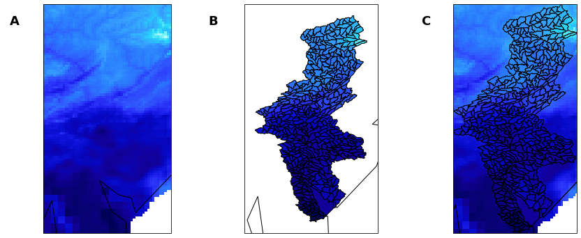
../../_images/gridmet_example.png — Fig. 2 Example grid-to-polygon interpolation of Gridmet data. A) Gridded Daily Maximum Temperature from Gridmet dataset. B) Huc12 basins for Delaware River Watershed C) Area-weighted-average interpolation of gridded Gridmet data to Huc12 polygons.#

References#

[ADPH18]

John T. Abatzoglou, Solomon Z. Dobrowski, Sean A. Parks, and Katherine C. Hegewisch. TerraClimate, a high-resolution global dataset of monthly climate and climatic water balance from 1958–2015. Scientific Data, January 2018. URL: https://doi.org/10.1038/sdata.2017.191, doi:10.1038/sdata.2017.191.

[Blo22]

David Blodgett. Hydro-Network Linked Data Index. 2022. URL: https://waterdata.usgs.gov/blog/nldi-intro/.

[CLL21]

Taher Chegini, Hong-Yi Li, and L. Ruby Leung. Hyriver: hydroclimate data retriever. Journal of Open Source Software, 6(66):3175, 2021. URL: https://doi.org/10.21105/joss.03175, doi:10.21105/joss.03175.

[Joh23]

Mike Johnson. climateR-catalog. 2023. URL: mikejohnson51/climateR-catalogs.

import warnings

import hvplot.pandas
import hvplot.xarray
import holoviews as hv
import numpy as np
import pandas as pd
import xarray as xr
from pynhd import NLDI, WaterData
from pygeohydro import watershed

from gdptools import AggGen, ClimRCatData, WeightGen

pd.set_option("display.max_rows", None)
pd.set_option("display.max_columns", None)
pd.set_option("display.width", 1000)
pd.set_option("display.colheader_justify", "center")
pd.set_option("display.precision", 3)

warnings.filterwarnings("ignore")

Create GeoDataFrame of Delaware River Basin HUC12s#

In this cell we use clients to several https://api.water.usgs.gov tools:

Tool: USGS NLDI Client: pynhd.NLDI
Tool: USGS GeoServer Client: pynhd.WaterData

More examples of using the HyRiver pynhd package can be found here

# Delaware River Basin HUC12s
# --------------------------------
wbd = watershed.WBD("huc4")
delaware_basin = wbd.byids(field="huc4", fids="0204")
huc12_basins = WaterData("wbd12").bybox(delaware_basin.iloc[0].geometry.bounds)
huc12_basins = huc12_basins[huc12_basins["huc12"].str.startswith(("020401", "020402"))]
huc12_basins.head()

Create a plot of the HUC12 Basins.

from holoviews.element.tiles import EsriTerrain

drb = huc12_basins.hvplot(
    geo=True,
    coastline="50m",
    alpha=0.2,
    c="r",
    frame_width=300,
    xlabel="longitude",
    ylabel="latitude",
    title="Delaware River HUC12 basins",
    xlim=(-76.8, -73.8),
    aspect="equal",
)
EsriTerrain() * drb

Query the climateR-catalog#

The variables tmmn, tmmx, pr, are available in the Gridmet dataset. Pandas is used to query the dataset.

In the following steps the json catalog files are imported into pandas.
Using the pandas query function to search for the Gridmet dataset for each variable of interest and return the json metadata for the parameter and grid catalog entries.

climater_cat = "https://github.com/mikejohnson51/climateR-catalogs/releases/download/June-2024/catalog.parquet"
cat = pd.read_parquet(climater_cat)
cat.head()

Pandas query function example#

_id = "gridmet"
_varname = "tmmx"

# an example query returns a pandas dataframe.
tc = cat.query("id == @_id & variable == @_varname")
tc

Query the climateR-catalog for variables tmmx, tmmn, pr#

Query the catalog for each variable of interest. The pandas query() function returns a pandas DataFrame but we want just the dictionary representation of the catalog entry so it’s converted to a dictionary with format dict[str, dict[str, Any]], where the first key is the variable of interest and the value is a dictionary of the resulting climateR-catalog data.

# Create a dictionary of parameter dataframes for each variable
tvars = ["tmmx", "tmmn", "pr"]
cat_params = [cat.query("id == @_id & variable == @_var").to_dict(orient="records")[0] for _var in tvars]

cat_dict = dict(zip(tvars, cat_params))

# Output an example of the cat_param entry for "pr".
cat_dict.get("pr")

Calculate the weights that will be used in the area-weighted statistics#

A note on the methods applied here:

There are currently three data classes, ClimRCatData, for use with input data derived from the climateR-catalog, NHGFStacData, for use with input data derived from the NHGF STAC catalog, and UserCatData for user-defined input data. The non-catalog examples demonstrate the use of UserCatData, and here ClimRCatData is demonstrated.

WeightGen() is the tool for generating weights. There are several methods available including: “serial”, “parallel”, and “dask”. If generating weights over a scale similar to the DRB huc12 basins here, serial using the serial method is appropriate. If for example weights are generated for huc12 basins over all of CONUS then “parallel” or “dask” (if you have a dask cluster available) will provide a significant speed-up.

The calculate_weights() method has the option to set interesection=True, which will save the intersected polygon geometries to wght_gen and the can be retrieved with the wght_gen.intersections property. We set it to True here so we could use it to evaluate the calculated weights and resulting aggregated values later in this notebook. Normally, one could just calculate weights() and the default value for intersections is False.

user_data = ClimRCatData(
    source_cat_dict=cat_dict,
    target_gdf=huc12_basins,
    target_id="huc12",
    source_time_period=["1980-01-01", "1980-12-31"],
)

wght_gen = WeightGen(
    user_data=user_data, method="serial", output_file="gridmet_daily_wghts.csv", weight_gen_crs=6931
)

wghts = wght_gen.calculate_weights(intersections=True)

Returned weights dataframe#

wghts.head()

Calculate the area-weighted averages#

For each variable in the Gridmet dataset and for each HUC12 in the Delaware River basin
Output the result as a netcdf file.
The data can also be output as a .csv file.

Returned values#

ngdf: The original huc12_basins geodataframe is sorted by user_data.id_feature, and dissolved by user_data.id_feature. So the returned geodataframe is a modified version of the original huc12_basins, and is returned for easy evaluation and for plotting.
ds_out: Xarray dataset representing the aggregated values and dimensioned by (time, user_data.id_feature). Again return for evaluation and plotting purposes.

properties#

agg_data. The user_data prepared for aggregating. Can be used to get the gridded dataset subsetted by time and feature bounding box.

agg_gen = AggGen(
    user_data=user_data,
    stat_method="masked_mean",
    agg_engine="serial",
    agg_writer="netcdf",
    weights="gridmet_daily_wghts.csv",
    out_path=".",
    file_prefix="testing_gridmet_drb_huc12",
)
ngdf, ds_out = agg_gen.calculate_agg()

Return the subset of gridMET data#

agg_gen prepares the user_data by subsetting the gridded data by the bounding box of the user.feature data and the user_data.period. This prepared data is available via the agg_gen.agg_data property. The return value is a dict[var, AggData]. To retrieve the prepared data, use the get() method on the dict by variable. The da property is the sub-setted xarray DataArray of the variable “tmmx” (daily maximum temperature).

processed_data = agg_gen.agg_data
da = processed_data.get("tmmx").da
da

Plot the resulting interpolation#

Calulate min/max of value and time=7 to adjust plotting paramters below

var = "daily_maximum_temperature"
time_step = "1980-08-01"

vmin = np.nanmin(da.sel(day=time_step).values)
vmax = np.nanmax(da.sel(day=time_step).values)
print(vmin, vmax)

ngdf[var] = ds_out[var].sel(time=time_step)
gridmet_agg = ngdf.to_crs(4326).hvplot(
    c=var,
    geo=True,
    coastline="50m",
    frame_width=300,
    alpha=1,
    cmap="viridis",
    clim=(vmin, vmax),
    xlabel="longitude",
    ylabel="latitude",
    clabel="daily maximum temperature (K)",
    xlim=(-76.8, -73.8),
    title="DRB HUC12 area-weighted average",
    aspect="equal",
)
gridmet_raw = da.sel(day=time_step).hvplot.quadmesh(
    "lon",
    "lat",
    var,
    cmap="viridis",
    alpha=1,
    grid=True,
    geo=True,
    coastline="50m",
    frame_width=300,
    clim=(vmin, vmax),
    xlabel="longitude",
    ylabel="latitude",
    clabel="daily maximum temperature (K)",
    xlim=(-76.8, -73.8),
    title="gridMET Daily Maximum Temperature",
    aspect="equal",
)

plot = (
    (EsriTerrain() * gridmet_raw) + (EsriTerrain() * gridmet_agg) + (EsriTerrain() * gridmet_raw * gridmet_agg)
)
plot

# Uncomment to save image above
# # Generate PNG plot using matplotlib backend (no browser required)
# import os

# import matplotlib

# matplotlib.use("Agg")  # Use non-interactive backend

# # Ensure the assets directory exists for documentation
# assets_dir = "../../assets"
# os.makedirs(assets_dir, exist_ok=True)

# try:
#     # First try to save with matplotlib backend
#     hv.extension("matplotlib")

#     hv.save(plot, f"{assets_dir}/gridmet_example.png", backend="matplotlib")
#     print(f"✓ Plot saved successfully to {assets_dir}/gridmet_example.png using matplotlib backend")

# except Exception as e:
#     print(f"HoloViews matplotlib failed: {e}")

Inspect structure of saved netcdf file#

ncf = xr.open_dataset("testing_gridmet_drb_huc12.nc")
ncf

Validation of area-weighted mean#

In the following sections we use some helper functions, which return information on the intersection calculation to create an illustration of the resulting intersection and calculated value at a polygon within the huc12_basins geodataframe.

The analysis is performed on one of the huc12_basins polygons using the huc12 id - “020402060505”. It extracts the grid_cells intersected by the huc12 polygon, the resulting intersections of the grid_cells with the huc12 polygon, and the aggregated value of the huc12 polygon for one of the days in the resulting aggregation.

grid_cells (GeoDataFrame): The polygons representing each cell of the gridMET grid.
intersections (GeoDataFrame): The grid_cells intersections with the huc12_basins polygons.
ngdf_poly (GeoDataFrame): The resorted and dissolved GeoDataFrame from agg_gen.
weights (xarray.Dataset): The generated weights read into xarray Dataset.

time = 7
huc12_id = "020402060505"
grid_cells = wght_gen.grid_cells

weights = pd.read_csv("gridmet_daily_wghts.csv").groupby("huc12").get_group(int(huc12_id))
i_ind = weights.i.values
j_ind = weights.j.values
wght = weights.wght.values

i_max = max(i_ind)
i_min = min(i_ind)
j_max = max(j_ind)
j_min = min(j_ind)

tmp = [grid_cells.query("i_index == @i and j_index == @j") for i, j in zip(i_ind, j_ind, strict=False)]
grid_cell_sub = pd.concat(tmp)

tmax_vals = da.values[:, i_ind, j_ind]
grid_cell_sub[var] = tmax_vals[time]
min_val = min(grid_cell_sub[var].values)
max_val = max(grid_cell_sub[var].values)
grid_cell_sub

inter_sect_sub = wght_gen.intersections.groupby("huc12").get_group(huc12_id)
inter_sect_sub.to_crs(4326, inplace=True)
inter_sect_sub.reset_index(drop=True, inplace=True)
inter_sect_sub[var] = tmax_vals[time]
inter_sect_sub["wght"] = wght

ngdf_poly = ngdf.groupby("huc12").get_group("020402060505")


aggvals = xr.open_dataset("testing_gridmet_drb_huc12.nc")
huc12_index = np.where(aggvals.huc12.values == huc12_id)[0][0]
ngdf_poly[var] = aggvals[var].values[time, huc12_index]

grid_cell_sub[var] = da.values[time, i_ind, j_ind]
inter_sect_sub[var] = da.values[time, i_ind, j_ind]
ngdf_poly[var] = aggvals[var].values[time, huc12_index]
min_val = min(grid_cell_sub[var].values)
max_val = max(grid_cell_sub[var].values)

print(grid_cell_sub.crs, ngdf_poly.crs, inter_sect_sub.crs)

grid_cell_sub.to_crs(4326, inplace=True)
ngdf_poly.to_crs(4326, inplace=True)

Plot the results#

Create labels:
- inter_sect_sub: for each intersection, determine the centroid of the cell to position the label. The text of the label will be the weight corresponding to the intersected area.
- grid_cell_sub: For each grid cell determine the centroid of the cell to position the label. The text of the label will be the tmmx value associated with the time variable.
- ngdf_poly: Determine the centroid of the polygon to position the label. The text of the label is the aggregated value for the time and huc12_id.
Create plots: Use hvplot to create plots of the 3 geodataframes and add the corresponding labels to each of the three figures.

for idx, row in inter_sect_sub.iterrows():
    cent = row.geometry.centroid
    inter_sect_sub.at[idx, "lon"] = cent.x
    inter_sect_sub.at[idx, "lat"] = cent.y
is_labels = inter_sect_sub.hvplot.labels(x="lon", y="lat", text="wght", text_color="r", text_baseline="center")

for idx, row in grid_cell_sub.iterrows():
    cent = row.geometry.centroid
    grid_cell_sub.at[idx, "lon"] = cent.x
    grid_cell_sub.at[idx, "lat"] = cent.y
grd_labels = grid_cell_sub.hvplot.labels(x="lon", y="lat", text=var, text_color="black", text_baseline="center")

for idx, row in ngdf_poly.iterrows():
    cent = row.geometry.centroid
    ngdf_poly.at[idx, "lon"] = cent.x
    ngdf_poly.at[idx, "lat"] = cent.y
ngdf_labels = ngdf_poly.hvplot.labels(x="lon", y="lat", text=var, text_color="black", text_baseline="center")

from holoviews import opts

gc_p = grid_cell_sub.hvplot(c=var, cmap="viridis", clim=(min_val, max_val))
int_p = inter_sect_sub.hvplot(c=var, cmap="viridis", clim=(min_val, max_val))
gdf_p = ngdf_poly.hvplot(c=var, cmap="viridis", clim=(min_val, max_val))

layout = ((gc_p * grd_labels) + (int_p * is_labels) + (gdf_p * ngdf_labels)).cols(1)
layout.opts(opts.Layout(shared_axes=True))

np.sum(grid_cell_sub[var].values * inter_sect_sub.wght.values)