Zonal statistics of rasters#
Deprecation Notice: The
serial,parallel, anddaskzonal engines are deprecated and will be removed in a future version. Usezonal_engine="exactextract"instead — it provides better performance and handles large datasets with bounded memory. See the ExactExtract Engine section below.
import geopandas as gpd
import pandas as pd
import rioxarray as rxr
import xarray as xr

from gdptools import ZonalGen
from gdptools.data.user_data import UserTiffData
# Be sure to use rioxarray to read tiff
rds_slope = rxr.open_rasterio("../../../tests/data/rasters/slope/slope.tif")
rds_text = rxr.open_rasterio("../../../tests/data/rasters/TEXT_PRMS/TEXT_PRMS.tif")
# Use geopandas to read shape file,
# Best if shape file only has feature id, and geometry if possible.
gdf = gpd.read_file("../../../tests/data/Oahu.shp")
id_feature = "fid"
print(len(gdf.groupby(id_feature)))
# These params are used to fill out the TiffAttributes class
tx_name= 'x'
ty_name = 'y'
band = 'band'
crs = 26904
varname = "slope" # not currently used
categorical = False # is the data categorical or not, if the data are integers it should
                   # probably be categorical.
data = UserTiffData(
    source_var=varname,
    source_ds=rds_slope,
    source_crs=crs,
    source_x_coord=tx_name,
    source_y_coord=ty_name,
    band=1,
    bname=band,
    target_gdf=gdf,
    target_id=id_feature
)

zonal_gen = ZonalGen(
    user_data=data,
    zonal_engine="serial",
    zonal_writer="csv",
    out_path=".",
    file_prefix="Oahu_slope_stats"
)
stats = zonal_gen.calculate_zonal(categorical=categorical)
print(stats)

# stats = zonal_gen.calculate_zonal(categorical=True)
# print(stats)
304
          count       mean        std  min    25%   50%   75%   max     sum
fid
1104.0  20431.0   1.872155   3.757167  0.0   0.00   0.0   1.0  32.0   38250
1105.0   2388.0  26.350921  13.473957  5.0  14.00  24.0  37.0  61.0   62926
1106.0   3192.0  33.687030  14.188686  1.0  22.00  34.0  45.0  70.0  107529
1107.0   6600.0  23.704091  15.854788  0.0  10.00  21.0  37.0  66.0  156447
1108.0  11380.0  22.116169  14.062708  0.0  11.00  21.0  33.0  62.0  251682
...         ...        ...        ...  ...    ...   ...   ...   ...     ...
1403.0   2753.0   1.722121   3.183146  0.0   0.00   1.0   1.0  23.0    4741
1404.0     99.0   1.363636   1.082840  0.0   0.00   2.0   2.0   3.0     135
1405.0    174.0  10.505747   7.044653  0.0   5.25   9.0  14.0  32.0    1828
1406.0   3089.0  10.931693  10.120911  0.0   4.00   7.0  15.0  59.0   33768
1407.0    321.0   1.679128   1.702893  0.0   1.00   1.0   2.0   9.0     539

[304 rows x 9 columns]
gdf.sort_values(by=id_feature, inplace=True)
stats.sort_values(by=id_feature, inplace=True)
gdf["slope_mean"] = stats["mean"].values
gdf
| fid | rpu | cat_id | hru_segmen | geometry | slope_mean | |
|---|---|---|---|---|---|---|
| 0 | 1104.0 | f | 1104 | 995.0 | POLYGON ((601200 2359860, 601180.267 2359853.7... | 1.872155 |
| 1 | 1105.0 | f | 1105 | 996.0 | POLYGON ((593760 2369060, 593675.2 2369014.8, ... | 26.350921 |
| 2 | 1106.0 | f | 1106 | 997.0 | POLYGON ((615055.367 2375324.633, 615130.633 2... | 33.687030 |
| 3 | 1107.0 | f | 1107 | 998.0 | POLYGON ((619150 2380290, 619096.633 2380263.3... | 23.704091 |
| 4 | 1108.0 | f | 1108 | 999.0 | POLYGON ((614640 2382950, 614628.833 2383001.1... | 22.116169 |
| ... | ... | ... | ... | ... | ... | ... |
| 299 | 1403.0 | f | 1403 | 1070.0 | POLYGON ((620198.262 2355012.754, 620153.3 235... | 1.722121 |
| 300 | 1404.0 | f | 1404 | 1029.0 | POLYGON ((579986.031 2380993.933, 580280 23810... | 1.363636 |
| 301 | 1405.0 | f | 1405 | 1146.0 | POLYGON ((625200 2365570, 625207.872 2365555.4... | 10.505747 |
| 302 | 1406.0 | f | 1406 | 1146.0 | POLYGON ((625144.965 2365356.034, 625183.9 236... | 10.931693 |
| 303 | 1407.0 | f | 1407 | 1233.0 | POLYGON ((618131.067 2357417.7, 618105.367 235... | 1.679128 |
304 rows × 6 columns
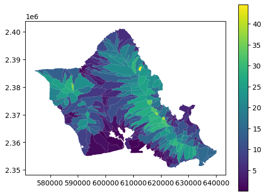
gdf.plot(column="slope_mean", legend=True)
<Axes: >
Parallel generator#
In this case the generator is slower because the domain is small and the overhead of generating the parallel processes takes more time than the actual calculation. However with a large domain the “parallel” zonal_engine is faster and has a smaller memory footprint.
zonal_gen2 = ZonalGen(
    user_data=data,
    zonal_engine="parallel",
    zonal_writer="csv",
    out_path=".",
    file_prefix="Oahu_slope_stats_p",
    jobs=2
)
stats = zonal_gen2.calculate_zonal(categorical=categorical)
print(stats)
          count       mean        std  min    25%   50%   75%   max     sum
fid
1104.0  20431.0   1.872155   3.757167  0.0   0.00   0.0   1.0  32.0   38250
1105.0   2388.0  26.350921  13.473957  5.0  14.00  24.0  37.0  61.0   62926
1106.0   3192.0  33.687030  14.188686  1.0  22.00  34.0  45.0  70.0  107529
1107.0   6600.0  23.704091  15.854788  0.0  10.00  21.0  37.0  66.0  156447
1108.0  11380.0  22.116169  14.062708  0.0  11.00  21.0  33.0  62.0  251682
...         ...        ...        ...  ...    ...   ...   ...   ...     ...
1403.0   2753.0   1.722121   3.183146  0.0   0.00   1.0   1.0  23.0    4741
1404.0     99.0   1.363636   1.082840  0.0   0.00   2.0   2.0   3.0     135
1405.0    174.0  10.505747   7.044653  0.0   5.25   9.0  14.0  32.0    1828
1406.0   3089.0  10.931693  10.120911  0.0   4.00   7.0  15.0  59.0   33768
1407.0    321.0   1.679128   1.702893  0.0   1.00   1.0   2.0   9.0     539

[304 rows x 9 columns]
gdf.sort_values(by=id_feature, inplace=True)
stats.sort_values(by=id_feature, inplace=True)
gdf["slope_mean"] = stats["mean"].values
gdf
| fid | rpu | cat_id | hru_segmen | geometry | slope_mean | |
|---|---|---|---|---|---|---|
| 0 | 1104.0 | f | 1104 | 995.0 | POLYGON ((601200 2359860, 601180.267 2359853.7... | 1.872155 |
| 1 | 1105.0 | f | 1105 | 996.0 | POLYGON ((593760 2369060, 593675.2 2369014.8, ... | 26.350921 |
| 2 | 1106.0 | f | 1106 | 997.0 | POLYGON ((615055.367 2375324.633, 615130.633 2... | 33.687030 |
| 3 | 1107.0 | f | 1107 | 998.0 | POLYGON ((619150 2380290, 619096.633 2380263.3... | 23.704091 |
| 4 | 1108.0 | f | 1108 | 999.0 | POLYGON ((614640 2382950, 614628.833 2383001.1... | 22.116169 |
| ... | ... | ... | ... | ... | ... | ... |
| 299 | 1403.0 | f | 1403 | 1070.0 | POLYGON ((620198.262 2355012.754, 620153.3 235... | 1.722121 |
| 300 | 1404.0 | f | 1404 | 1029.0 | POLYGON ((579986.031 2380993.933, 580280 23810... | 1.363636 |
| 301 | 1405.0 | f | 1405 | 1146.0 | POLYGON ((625200 2365570, 625207.872 2365555.4... | 10.505747 |
| 302 | 1406.0 | f | 1406 | 1146.0 | POLYGON ((625144.965 2365356.034, 625183.9 236... | 10.931693 |
| 303 | 1407.0 | f | 1407 | 1233.0 | POLYGON ((618131.067 2357417.7, 618105.367 235... | 1.679128 |
304 rows × 6 columns
gdf.plot(column="slope_mean", legend=True)
<Axes: >
ExactExtract Engine (High Performance)#
gdptools now supports the exactextract engine, which provides 10-100x faster zonal statistics by operating directly on raster data without converting to vector polygons.
Engine Comparison#
Engine |
Status |
Description |
Best For |
Weighted Stats |
|---|---|---|---|---|
|
Recommended |
Raster-native C++ library |
Any size, fastest |
Planned (#94) |
|
Deprecated |
Single-threaded, vector-based |
Small datasets, debugging |
Yes |
|
Deprecated |
Multi-threaded via joblib |
Medium datasets |
Yes |
|
Deprecated |
Distributed via Dask cluster |
Very large datasets |
Yes |
Why is exactextract faster?#
Raster-native: Operates directly on raster blocks without creating polygon geometries
Coverage fractions: Computes cell coverage analytically (no expensive intersection calls)
Streaming: Processes raster blocks on-demand without full array materialization
C++ backend: Core algorithms implemented in optimized C++
Note: exactextract does not yet support weighted zonal statistics. Weighted support via exactextract’s built-in coverage fractions is planned in issue #94. Until then, the deprecated engines remain available for WeightedZonalGen.
import time

# Reload data for fair comparison
data_slope = UserTiffData(
    source_var="slope",
    source_ds=rds_slope,
    source_crs=crs,
    source_x_coord=tx_name,
    source_y_coord=ty_name,
    band=1,
    bname=band,
    target_gdf=gdf[[id_feature, "geometry"]].copy(),
    target_id=id_feature
)

# ExactExtract engine - fastest option
zonal_gen_exact = ZonalGen(
    user_data=data_slope,
    zonal_engine="exactextract",  # New high-performance engine!
    zonal_writer="csv",
    out_path=".",
    file_prefix="Oahu_slope_stats_exact"
)

start = time.perf_counter()
stats_exact = zonal_gen_exact.calculate_zonal(categorical=False)
exact_time = time.perf_counter() - start
print(f"\nexactextract completed in {exact_time:.4f} seconds")
print(stats_exact.head())
exactextract completed in 1.7003 seconds
               count       mean        std  min  25%  50%  75%  max  \
fid
1104.0  20413.586391   1.874860   3.758853    0    0    0    1   32
1105.0   2390.553052  26.282542  13.461160    0   14   23   36   61
1106.0   3195.079310  33.641735  14.204321    1   22   34   44   70
1107.0   6605.529560  23.720972  15.855884    0   10   21   37   66
1108.0  11364.951446  22.139100  14.065037    0   11   20   33   62

                  sum
fid
1104.0   38272.622751
1105.0   62829.811849
1106.0  107488.011195
1107.0  156689.583950
1108.0  251609.791194
Timing Comparison: All Engines#
Let’s compare the performance of all three engines on the same dataset:
timing_results = {}

# Serial engine
zonal_serial = ZonalGen(
    user_data=data_slope,
    zonal_engine="serial",
    zonal_writer="csv",
    out_path=".",
    file_prefix="timing_serial"
)
start = time.perf_counter()
_ = zonal_serial.calculate_zonal(categorical=False)
timing_results["serial"] = time.perf_counter() - start

# Parallel engine
zonal_parallel = ZonalGen(
    user_data=data_slope,
    zonal_engine="parallel",
    zonal_writer="csv",
    out_path=".",
    file_prefix="timing_parallel",
    jobs=4
)
start = time.perf_counter()
_ = zonal_parallel.calculate_zonal(categorical=False)
timing_results["parallel"] = time.perf_counter() - start

# ExactExtract engine
zonal_exact = ZonalGen(
    user_data=data_slope,
    zonal_engine="exactextract",
    zonal_writer="csv",
    out_path=".",
    file_prefix="timing_exact"
)
start = time.perf_counter()
_ = zonal_exact.calculate_zonal(categorical=False)
timing_results["exactextract"] = time.perf_counter() - start

# Display results
print("\n" + "="*50)
print("TIMING COMPARISON")
print("="*50)
for engine, t in timing_results.items():
    speedup = timing_results["serial"] / t
    print(f"{engine:15} : {t:8.4f} sec  ({speedup:5.1f}x vs serial)")
print("="*50)
==================================================
TIMING COMPARISON
==================================================
serial          :   2.0848 sec  (  1.0x vs serial)
parallel        :   4.2354 sec  (  0.5x vs serial)
exactextract    :   1.6783 sec  (  1.2x vs serial)
==================================================
Key Takeaways#
exactextract is the recommended engine — typically 10-100x faster than vector-based engines because it operates directly on raster blocks without constructing intersection geometries.
The serial, parallel, and dask engines are deprecated and will be removed in a future version.
Use exactextract for all new zonal statistics work (mean, sum, min, max, etc.).
Weighted zonal statistics via exactextract are planned (issue #94). Until then,
WeightedZonalGenstill uses the deprecated engines.
varname = "TEXT" # not currently used
categorical = True # is the data categorical or not, if the data are integers it should
                   # probably be categorical.
data = UserTiffData(
    source_var=varname,
    source_ds=rds_text,  # Use rds_text for categorical example
    source_crs=crs,
    source_x_coord=tx_name,
    source_y_coord=ty_name,
    band=1,
    bname=band,
    target_gdf=gdf,
    target_id=id_feature
)

zonal_gen = ZonalGen(
    user_data=data,
    zonal_engine="serial",
    zonal_writer="csv",
    out_path=".",
    file_prefix="Oahu_TEXT_stats"
)
stats = zonal_gen.calculate_zonal(categorical=categorical)
print(stats)
          0    1         2         3  count
fid
1104.0  0.0  0.0  0.654237  0.345763    295
1105.0  0.0  0.0  0.882353  0.117647     34
1106.0  0.0  0.0  0.979167  0.020833     48
1107.0  0.0  0.0  0.191489  0.808511     94
1108.0  0.0  0.0  0.197605  0.802395    167
...     ...  ...       ...       ...    ...
1298.0  0.0  0.0  0.186047  0.813953     43
1307.0  0.0  0.0  0.841818  0.158182    550
1377.0  0.0  0.0  0.844660  0.155340    103
1389.0  0.0  0.0  1.000000  0.000000     20
1401.0  0.0  0.0  0.609756  0.390244     41

[304 rows x 5 columns]
# Compute the max category for each `fid`
max_category_df = stats.iloc[:, :-1].idxmax(axis=1).reset_index()
max_category_df.columns = ['fid', 'max_category']
# Merge the max category result into the GeoDataFrame
gdf = gdf.merge(max_category_df, on='fid', how='left')
gdf
| fid | rpu | cat_id | hru_segmen | geometry | slope_mean | max_category | |
|---|---|---|---|---|---|---|---|
| 0 | 1104.0 | f | 1104 | 995.0 | POLYGON ((601200 2359860, 601180.267 2359853.7... | 1.872155 | 2 |
| 1 | 1105.0 | f | 1105 | 996.0 | POLYGON ((593760 2369060, 593675.2 2369014.8, ... | 26.350921 | 2 |
| 2 | 1106.0 | f | 1106 | 997.0 | POLYGON ((615055.367 2375324.633, 615130.633 2... | 33.687030 | 2 |
| 3 | 1107.0 | f | 1107 | 998.0 | POLYGON ((619150 2380290, 619096.633 2380263.3... | 23.704091 | 3 |
| 4 | 1108.0 | f | 1108 | 999.0 | POLYGON ((614640 2382950, 614628.833 2383001.1... | 22.116169 | 3 |
| ... | ... | ... | ... | ... | ... | ... | ... |
| 299 | 1403.0 | f | 1403 | 1070.0 | POLYGON ((620198.262 2355012.754, 620153.3 235... | 1.722121 | 2 |
| 300 | 1404.0 | f | 1404 | 1029.0 | POLYGON ((579986.031 2380993.933, 580280 23810... | 1.363636 | 2 |
| 301 | 1405.0 | f | 1405 | 1146.0 | POLYGON ((625200 2365570, 625207.872 2365555.4... | 10.505747 | 2 |
| 302 | 1406.0 | f | 1406 | 1146.0 | POLYGON ((625144.965 2365356.034, 625183.9 236... | 10.931693 | 2 |
| 303 | 1407.0 | f | 1407 | 1233.0 | POLYGON ((618131.067 2357417.7, 618105.367 235... | 1.679128 | 2 |
304 rows × 7 columns
gdf.plot(column="max_category", legend=True)
<Axes: >

Parallel engine#
zonal_gen2 = ZonalGen(
    user_data=data,
    zonal_engine="parallel",
    zonal_writer="csv",
    out_path=".",
    file_prefix="Oahu_TEXT_stats",
    jobs=2
)
stats = zonal_gen2.calculate_zonal(categorical=categorical)
print(stats)
          0    1         2         3  count
fid
1104.0  0.0  0.0  0.654237  0.345763    295
1105.0  0.0  0.0  0.882353  0.117647     34
1106.0  0.0  0.0  0.979167  0.020833     48
1107.0  0.0  0.0  0.191489  0.808511     94
1108.0  0.0  0.0  0.197605  0.802395    167
...     ...  ...       ...       ...    ...
1298.0  0.0  0.0  0.186047  0.813953     43
1307.0  0.0  0.0  0.841818  0.158182    550
1377.0  0.0  0.0  0.844660  0.155340    103
1389.0  0.0  0.0  1.000000  0.000000     20
1401.0  0.0  0.0  0.609756  0.390244     41

[304 rows x 5 columns]
# Compute the max category for each `fid`
max_category_df = stats.iloc[:, :-1].idxmax(axis=1).reset_index()
max_category_df.columns = ['fid', 'max_category_p']

gdf = gdf.merge(max_category_df, on='fid', how='left')
gdf
| fid | rpu | cat_id | hru_segmen | geometry | slope_mean | max_category | max_category_p | |
|---|---|---|---|---|---|---|---|---|
| 0 | 1104.0 | f | 1104 | 995.0 | POLYGON ((601200 2359860, 601180.267 2359853.7... | 1.872155 | 2 | 2 |
| 1 | 1105.0 | f | 1105 | 996.0 | POLYGON ((593760 2369060, 593675.2 2369014.8, ... | 26.350921 | 2 | 2 |
| 2 | 1106.0 | f | 1106 | 997.0 | POLYGON ((615055.367 2375324.633, 615130.633 2... | 33.687030 | 2 | 2 |
| 3 | 1107.0 | f | 1107 | 998.0 | POLYGON ((619150 2380290, 619096.633 2380263.3... | 23.704091 | 3 | 3 |
| 4 | 1108.0 | f | 1108 | 999.0 | POLYGON ((614640 2382950, 614628.833 2383001.1... | 22.116169 | 3 | 3 |
| ... | ... | ... | ... | ... | ... | ... | ... | ... |
| 299 | 1403.0 | f | 1403 | 1070.0 | POLYGON ((620198.262 2355012.754, 620153.3 235... | 1.722121 | 2 | 2 |
| 300 | 1404.0 | f | 1404 | 1029.0 | POLYGON ((579986.031 2380993.933, 580280 23810... | 1.363636 | 2 | 2 |
| 301 | 1405.0 | f | 1405 | 1146.0 | POLYGON ((625200 2365570, 625207.872 2365555.4... | 10.505747 | 2 | 2 |
| 302 | 1406.0 | f | 1406 | 1146.0 | POLYGON ((625144.965 2365356.034, 625183.9 236... | 10.931693 | 2 | 2 |
| 303 | 1407.0 | f | 1407 | 1233.0 | POLYGON ((618131.067 2357417.7, 618105.367 235... | 1.679128 | 2 | 2 |
304 rows × 8 columns
gdf.plot(column="max_category_p", legend=True)
<Axes: >
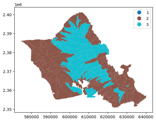
ExactExtract Engine with Categorical Data#
The exactextract engine also supports categorical zonal statistics with the categorical=True parameter. For categorical data, it computes the count/area of each unique category within each polygon.
# Set up categorical data using TEXT raster
data_text = UserTiffData(
    source_var="TEXT",
    source_ds=rds_text,
    source_crs=crs,
    source_x_coord=tx_name,
    source_y_coord=ty_name,
    band=1,
    bname=band,
    target_gdf=gdf[[id_feature, "geometry"]].copy(),
    target_id=id_feature
)

# ExactExtract engine with categorical data
zonal_gen_exact_cat = ZonalGen(
    user_data=data_text,
    zonal_engine="exactextract",
    zonal_writer="csv",
    out_path=".",
    file_prefix="Oahu_TEXT_stats_exact"
)

start = time.perf_counter()
stats_exact_cat = zonal_gen_exact_cat.calculate_zonal(categorical=True)
exact_cat_time = time.perf_counter() - start
print(f"\nexactextract (categorical) completed in {exact_cat_time:.4f} seconds")
print(stats_exact_cat.head())
exactextract (categorical) completed in 1.4251 seconds
          0    1         2         3  count
fid
1104.0  0.0  0.0  0.653648  0.346352    294
1105.0  0.0  0.0  0.857603  0.142397     34
1106.0  0.0  0.0  0.985308  0.014692     46
1107.0  0.0  0.0  0.199234  0.800766     95
1108.0  0.0  0.0  0.198175  0.801825    164
# Compute the max category for each polygon
max_category_exact = stats_exact_cat.iloc[:, :-1].idxmax(axis=1).reset_index()
max_category_exact.columns = ['fid', 'max_category_exact']

# Merge into GeoDataFrame and plot
gdf = gdf.merge(max_category_exact, on='fid', how='left')
gdf.plot(column="max_category_exact", legend=True)
<Axes: >