NHGF STAC Catalog - NLCD Land Cover Zonal Statistics Example#
This example demonstrates how to use GeoTIFF-backed STAC collections with
gdptools. While the CONUS404 example works
with Zarr time-series data, the NHGF STAC catalog also contains collections
stored as individual GeoTIFF files — one per time step.
Here we compute categorical zonal statistics of NLCD (National Land Cover Database) land cover classes for HUC12 basins in the Delaware River Basin.
Key Differences from Zarr Workflow#
Zarr (e.g., CONUS404) |
GeoTIFF (e.g., NLCD) |
|
|---|---|---|
Asset type |
Single |
One |
Time dimension |
|
No time dimension — one raster per year |
|
Selects a time range from the Zarr store |
Selects which STAC item (year) to use |
Typical analysis |
Area-weighted temporal aggregation |
Zonal statistics (categorical or continuous) |
NHGFStacData auto-detects the collection format and returns the appropriate
handler (NHGFStacZarrData or NHGFStacTiffData) transparently.
import warnings

import geopandas as gpd
import hvplot.pandas
from pygeohydro import watershed
from pynhd import WaterData

from gdptools import NHGFStacData, ZonalGen
from gdptools.helpers import get_stac_collection

warnings.filterwarnings("ignore")
Load the Target Polygons#
We use the same Delaware River Basin HUC12 polygons as the CONUS404 example.
These are retrieved from the Watershed Boundary Dataset (WBD) via pygeohydro.
wbd = watershed.WBD("huc4")
delaware_basin = wbd.byids(field="huc4", fids="0204")
huc12_basins = WaterData("wbd12").bygeom(delaware_basin.iloc[0].geometry)
huc12_basins = huc12_basins[
    huc12_basins["huc12"].str.startswith(("020401", "020402"))
]
huc12_basins.head()
| geometry | tnmid | metasourceid | sourcedatadesc | sourceoriginator | sourcefeatureid | loaddate | gnis_id | areaacres | areasqkm | states | huc12 | name | hutype | humod | tohuc | noncontributingareaacres | noncontributingareasqkm | globalid | |
|---|---|---|---|---|---|---|---|---|---|---|---|---|---|---|---|---|---|---|---|
| 0 | MULTIPOLYGON (((-75.02421 39.44397, -75.02353 ... | {001055CD-7B5E-4F96-ABB1-22923FD2B454} | NaN | None | None | None | 2013-01-18T07:08:41Z | None | 16178.10 | 65.47 | NJ | 020402060505 | White Marsh Run-Maurice River | S | NM | 020402060507 | 0 | 0 | {A70A97FA-E29C-11E2-8094-0021280458E6} |
| 1 | MULTIPOLYGON (((-74.62113 41.00565, -74.62139 ... | {009DA440-393A-46A0-BBA3-C38139823414} | {ED602145-9201-4827-9CE1-05D252484579} | None | None | None | 2017-10-03T20:11:06Z | None | 29107.93 | 117.80 | NJ | 020401050502 | Lubbers Run-Musconetcong River | S | NM | 020401050503 | 0 | 0 | {B830B4F8-E29C-11E2-8094-0021280458E6} |
| 2 | MULTIPOLYGON (((-75.75805 40.65996, -75.75783 ... | {00F73634-FA00-464F-93F0-F0BCCB464567} | {ED602145-9201-4827-9CE1-05D252484579} | None | None | None | 2017-10-03T20:10:58Z | None | 35229.84 | 142.57 | PA | 020402030305 | Upper Maiden Creek | S | NM | 020402030307 | 0 | 0 | {BAF5E77A-E29C-11E2-8094-0021280458E6} |
| 3 | MULTIPOLYGON (((-75.13279 39.88601, -75.13439 ... | {017B8A58-E959-4600-B212-8EB921F0F9F7} | {E9F5C988-2313-440E-A05E-C5871E2773A6} | None | None | None | 2017-10-03T20:11:04Z | None | 24920.90 | 100.85 | NJ,PA | 020402020507 | Woodbury Creek-Delaware River | S | TF | 020402020607 | 0 | 0 | {B122D6B7-E29C-11E2-8094-0021280458E6} |
| 4 | MULTIPOLYGON (((-74.92817 40.55256, -74.92833 ... | {01B4598B-0623-407F-9133-3040D99A8D1A} | {ED602145-9201-4827-9CE1-05D252484579} | None | None | None | 2017-10-03T20:10:52Z | None | 15086.80 | 61.05 | NJ | 020401050905 | Lockatong Creek | S | NM | 020401050908 | 0 | 0 | {A6AB04BE-E29C-11E2-8094-0021280458E6} |
Fetch the NLCD Land Cover Collection#
The NLCD data is organized under the nlcd parent collection in the STAC
catalog, with sub-collections for each product (e.g., nlcd-LndCov for land
cover). The helper get_stac_collection() searches recursively, so we can
request "nlcd-LndCov" directly.
Unlike Zarr collections, GeoTIFF collections have no collection-level data
assets. Instead, each STAC item represents a single year and contains a
tif-s3-osn asset pointing to the GeoTIFF on S3.
collection = get_stac_collection("nlcd-LndCov")
print(f"Collection: {collection.id}")
print(f"Collection-level assets: {list(collection.assets.keys())}")

# List the first few items (each item is one year of NLCD)
items = list(collection.get_items())
print(f"\nNumber of items: {len(items)}")
for item in items[:5]:
    print(f"  {item.id}  -  {item.properties.get('datetime')}")
Collection: nlcd-LndCov
Collection-level assets: []
Number of items: 40
  Annual_NLCD_LndCov_1985_CU_C1V1  -  1985-01-01T00:00:00Z
  Annual_NLCD_LndCov_1986_CU_C1V1  -  1986-01-01T00:00:00Z
  Annual_NLCD_LndCov_1987_CU_C1V1  -  1987-01-01T00:00:00Z
  Annual_NLCD_LndCov_1988_CU_C1V1  -  1988-01-01T00:00:00Z
  Annual_NLCD_LndCov_1989_CU_C1V1  -  1989-01-01T00:00:00Z
Create the NHGFStacData Object#
We pass the STAC collection to NHGFStacData just like the Zarr workflow.
The factory auto-detects that this is a GeoTIFF collection and returns an
NHGFStacTiffData instance.
source_time_periodselects the STAC item whose datetime falls in the given range (here, the 2021 NLCD product).source_varis the variable name used to label results.
user_data = NHGFStacData(
    source_collection=collection,
    source_var=["LndCov"],
    target_gdf=huc12_basins,
    target_id="huc12",
    source_time_period=["2021-01-01", "2021-12-31"],
)

print(f"Returned type: {type(user_data).__name__}")
print(f"Class type:    {user_data.get_class_type()}")
print(f"Source CRS:    {user_data.source_ds.rio.crs}")
Returned type: NHGFStacTiffData
Class type:    NHGFStacTiffData
Source CRS:    PROJCS["AEA        WGS84",GEOGCS["WGS 84",DATUM["WGS_1984",SPHEROID["WGS 84",6378137,298.257223563,AUTHORITY["EPSG","7030"]],AUTHORITY["EPSG","6326"]],PRIMEM["Greenwich",0],UNIT["degree",0.0174532925199433,AUTHORITY["EPSG","9122"]],AUTHORITY["EPSG","4326"]],PROJECTION["Albers_Conic_Equal_Area"],PARAMETER["latitude_of_center",23],PARAMETER["longitude_of_center",-96],PARAMETER["standard_parallel_1",29.5],PARAMETER["standard_parallel_2",45.5],PARAMETER["false_easting",0],PARAMETER["false_northing",0],UNIT["metre",1,AUTHORITY["EPSG","9001"]],AXIS["Easting",EAST],AXIS["Northing",NORTH]]
Compute Categorical Zonal Statistics#
NLCD land cover values are integers representing land cover classes (e.g.,
11 = Open Water, 21 = Developed Open Space, 41 = Deciduous Forest, etc.).
We use ZonalGen with categorical=True to compute the proportion of each
class within every HUC12 polygon.
zonal_gen = ZonalGen(
    user_data=user_data,
    zonal_engine="exactextract",
    zonal_writer="csv",
    out_path=".",
    file_prefix="drb_nlcd_2021",
)

stats = zonal_gen.calculate_zonal(categorical=True)
stats.head()
| 11 | 21 | 22 | 23 | 24 | 31 | 41 | 42 | 43 | 52 | 71 | 81 | 82 | 90 | 95 | 250 | count | |
|---|---|---|---|---|---|---|---|---|---|---|---|---|---|---|---|---|---|
| huc12 | |||||||||||||||||
| 020402060505 | 0.033158 | 0.085917 | 0.193784 | 0.122581 | 0.050119 | 0.018544 | 0.123280 | 0.023426 | 0.073461 | 0.010044 | 0.002161 | 0.009373 | 0.117233 | 0.114004 | 0.022915 | 0.0 | 72745 |
| 020401050502 | 0.023007 | 0.099705 | 0.065001 | 0.025624 | 0.006489 | 0.009425 | 0.637710 | 0.000275 | 0.005815 | 0.000620 | 0.007187 | 0.012210 | 0.007113 | 0.097954 | 0.001864 | 0.0 | 130884 |
| 020402030305 | 0.001496 | 0.065787 | 0.021263 | 0.007005 | 0.000548 | 0.000508 | 0.369402 | 0.000315 | 0.025328 | 0.001519 | 0.000303 | 0.185952 | 0.315260 | 0.005277 | 0.000038 | 0.0 | 158411 |
| 020402020507 | 0.220036 | 0.081773 | 0.194387 | 0.168000 | 0.140793 | 0.004056 | 0.038694 | 0.000054 | 0.001013 | 0.003698 | 0.002074 | 0.002793 | 0.016708 | 0.098271 | 0.027650 | 0.0 | 112057 |
| 020401050905 | 0.002738 | 0.072786 | 0.027082 | 0.009314 | 0.001413 | 0.000619 | 0.309156 | 0.000015 | 0.025494 | 0.004639 | 0.000472 | 0.340643 | 0.120848 | 0.083785 | 0.000996 | 0.0 | 67838 |
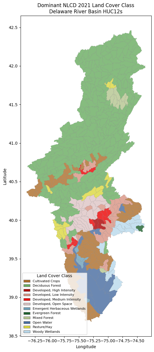
Identify the Dominant Land Cover Class#
For each HUC12 basin, find the NLCD class with the highest proportion and merge the result into the target GeoDataFrame for mapping.
# NLCD Land Cover class names
nlcd_classes = {
    "11": "Open Water",
    "12": "Perennial Ice/Snow",
    "21": "Developed, Open Space",
    "22": "Developed, Low Intensity",
    "23": "Developed, Medium Intensity",
    "24": "Developed, High Intensity",
    "31": "Barren Land",
    "41": "Deciduous Forest",
    "42": "Evergreen Forest",
    "43": "Mixed Forest",
    "52": "Shrub/Scrub",
    "71": "Grassland/Herbaceous",
    "81": "Pasture/Hay",
    "82": "Cultivated Crops",
    "90": "Woody Wetlands",
    "95": "Emergent Herbaceous Wetlands",
}

# NLCD official color palette
nlcd_colors = {
    "Open Water": "#466b9f",
    "Perennial Ice/Snow": "#d1def8",
    "Developed, Open Space": "#dec5c5",
    "Developed, Low Intensity": "#d99282",
    "Developed, Medium Intensity": "#eb0000",
    "Developed, High Intensity": "#ab0000",
    "Barren Land": "#b3ac9f",
    "Deciduous Forest": "#68ab5f",
    "Evergreen Forest": "#1c5f2c",
    "Mixed Forest": "#b5c58f",
    "Shrub/Scrub": "#ccb879",
    "Grassland/Herbaceous": "#dfdfc2",
    "Pasture/Hay": "#dbd83d",
    "Cultivated Crops": "#ab6c28",
    "Woody Wetlands": "#b8d9eb",
    "Emergent Herbaceous Wetlands": "#6c9fb8",
}

# Drop the 'count' column before finding the dominant class
class_cols = [c for c in stats.columns if c != "count"]
dominant = stats[class_cols].idxmax(axis=1).reset_index()
dominant.columns = ["huc12", "dominant_class"]

# Column names may be int or str — normalize to str before mapping
dominant["dominant_class"] = dominant["dominant_class"].astype(str).map(nlcd_classes)

gdf = huc12_basins.merge(dominant, on="huc12", how="left")

# Build a sorted color list matching the categories present in the data
categories = sorted(gdf["dominant_class"].dropna().unique())

gdf.head()
| geometry | tnmid | metasourceid | sourcedatadesc | sourceoriginator | sourcefeatureid | loaddate | gnis_id | areaacres | areasqkm | states | huc12 | name | hutype | humod | tohuc | noncontributingareaacres | noncontributingareasqkm | globalid | dominant_class | |
|---|---|---|---|---|---|---|---|---|---|---|---|---|---|---|---|---|---|---|---|---|
| 0 | MULTIPOLYGON (((-75.02421 39.44397, -75.02353 ... | {001055CD-7B5E-4F96-ABB1-22923FD2B454} | NaN | None | None | None | 2013-01-18T07:08:41Z | None | 16178.10 | 65.47 | NJ | 020402060505 | White Marsh Run-Maurice River | S | NM | 020402060507 | 0 | 0 | {A70A97FA-E29C-11E2-8094-0021280458E6} | Developed, Low Intensity |
| 1 | MULTIPOLYGON (((-74.62113 41.00565, -74.62139 ... | {009DA440-393A-46A0-BBA3-C38139823414} | {ED602145-9201-4827-9CE1-05D252484579} | None | None | None | 2017-10-03T20:11:06Z | None | 29107.93 | 117.80 | NJ | 020401050502 | Lubbers Run-Musconetcong River | S | NM | 020401050503 | 0 | 0 | {B830B4F8-E29C-11E2-8094-0021280458E6} | Deciduous Forest |
| 2 | MULTIPOLYGON (((-75.75805 40.65996, -75.75783 ... | {00F73634-FA00-464F-93F0-F0BCCB464567} | {ED602145-9201-4827-9CE1-05D252484579} | None | None | None | 2017-10-03T20:10:58Z | None | 35229.84 | 142.57 | PA | 020402030305 | Upper Maiden Creek | S | NM | 020402030307 | 0 | 0 | {BAF5E77A-E29C-11E2-8094-0021280458E6} | Deciduous Forest |
| 3 | MULTIPOLYGON (((-75.13279 39.88601, -75.13439 ... | {017B8A58-E959-4600-B212-8EB921F0F9F7} | {E9F5C988-2313-440E-A05E-C5871E2773A6} | None | None | None | 2017-10-03T20:11:04Z | None | 24920.90 | 100.85 | NJ,PA | 020402020507 | Woodbury Creek-Delaware River | S | TF | 020402020607 | 0 | 0 | {B122D6B7-E29C-11E2-8094-0021280458E6} | Open Water |
| 4 | MULTIPOLYGON (((-74.92817 40.55256, -74.92833 ... | {01B4598B-0623-407F-9133-3040D99A8D1A} | {ED602145-9201-4827-9CE1-05D252484579} | None | None | None | 2017-10-03T20:10:52Z | None | 15086.80 | 61.05 | NJ | 020401050905 | Lockatong Creek | S | NM | 020401050908 | 0 | 0 | {A6AB04BE-E29C-11E2-8094-0021280458E6} | Pasture/Hay |
Visualize the Results#
Map the dominant NLCD land cover class for each HUC12 basin in the Delaware River Basin.
import matplotlib.pyplot as plt
from matplotlib.patches import Patch

fig, ax = plt.subplots(figsize=(10, 12))
plot_gdf = gdf.to_crs(4326)

# Color each polygon by its NLCD class
colors = plot_gdf["dominant_class"].map(nlcd_colors).fillna("#cccccc")
plot_gdf.plot(ax=ax, color=colors, alpha=0.8, edgecolor="gray", linewidth=0.2)

# Build legend from classes present in the data
legend_handles = [
    Patch(facecolor=nlcd_colors[c], edgecolor="gray", label=c)
    for c in categories
]
ax.legend(
    handles=legend_handles,
    loc="lower left",
    fontsize=8,
    title="Land Cover Class",
)
ax.set_title("Dominant NLCD 2021 Land Cover Class\nDelaware River Basin HUC12s")
ax.set_xlabel("Longitude")
ax.set_ylabel("Latitude")
plt.tight_layout()