Area-Weighted Aggregation of Polygonal Datasets#
Using gdptools.WeightGenP2P — Intensive vs. Extensive Variables#
This notebook explains how to aggregate data from one set of polygons to another using area weights, focusing on the difference between intensive and extensive variables.
Intensive Variables#
Definition: Intensive variables are properties that do not depend on the size or area of a region. Their values do not add up when combining multiple regions.
Units: Expressed per unit area, per unit length, or per unit volume.
Behavior: When aggregating (combining or averaging) over a region, you calculate a weighted average (not a sum).
Examples:
Temperature: °C, K, °F
Precipitation rate: mm/hr, in/day
Concentration: mg/L, ppm
Population density: persons/km²
Key Point: Averaging or aggregating an intensive variable over a larger or smaller area does not change its units, and you must never add these values directly—instead, use an area-weighted mean.
Extensive Variables#
Definition: Extensive variables are properties that do depend on the size or area of a region. Their values do add up when combining regions.
Units: Expressed in raw quantities, not per area/length/volume.
Behavior: When aggregating over regions, you sum or proportionally allocate these variables.
Examples:
Population: persons
Total precipitation volume: m³
Total mass or load: kg, tons
Area: m², acres, hectares
Total streamflow (volume): m³/s (when integrated over time)
Total energy use: kWh
Key Point: When you combine two polygons, the extensive variables’ values sum directly, and their units are unchanged.
Comparison Table#
Variable Type |
Example Units |
Aggregation Behavior |
Typical Examples |
|---|---|---|---|
Intensive |
°C, mg/L, mm/hr, ppm |
Weighted average (not sum) |
Temperature, concentration, density |
Extensive |
persons, m³, kg |
Sum (proportional part) |
Population, total mass, area, flow |
How to Aggregate#
1. Intensive Variable Aggregation (e.g., Temperature, Population Density)#
Goal: Compute an area-weighted mean in the target polygon.
Where:
\(v_i\) is the value of the variable in source polygon \(i\) (units: \(U\), e.g., °C, mg/L, persons/km²)
\(a_i\) is the area of overlap between source polygon \(i\) and the target (units: \(\mathrm{m}^2\))
Units:#
Numerator: \(\sum v_i \times a_i = U \times \mathrm{m}^2\)
Denominator: \(\sum a_i = \mathrm{m}^2\)
So,
The units after aggregation are the same as the original intensive variable.
2. Extensive Variable Aggregation (e.g., Population, Total Load)#
Goal: Compute the area-weighted sum contributed by each source polygon to the target.
Formula (Area-Weighted Sum):#
Where:
\(V_i\) is the value of the extensive variable in source polygon \(i\) (units: \(U\), e.g., persons, kg)
\(a_i\) is the area of overlap between source polygon \(i\) and the target (units: \(\mathrm{m}^2\))
\(A_i\) is the total area of source polygon \(i\) (units: \(\mathrm{m}^2\))
Units:#
Fraction: \(\frac{a_i}{A_i}\) is unitless (\(\mathrm{m}^2 / \mathrm{m}^2\))
Each term: \(V_i \times \frac{a_i}{A_i} = U\)
Sum: \(\sum (U) = U\)
So,
The aggregated value has the same units as the original extensive variable.
Getting Started#
Directions for creating an environment to run this notebook.
Requirements:#
Conda-based package manager such as miniconda or mambaforge.
Create conda/mamba environment.#
Download environment-examples.yml
To create the conda environment follow the steps below:
conda env create -f environment-examples.yml
conda activate gdptools-examples
jupyter lab
2 Import Libraries and Create Sample Data#
import geopandas as gpd
import matplotlib.pyplot as plt
from shapely.geometry import Polygon

from gdptools import WeightGenP2P  # Adjust import if needed
# Define sample source polygons with an intensive variable (temperature)
# and an extensive variable (population).
source_polys = gpd.GeoDataFrame({
    'source_id': [1, 2],
    'temp': [10.0, 20.0],           # Intensive variable (e.g., temperature in °C)
    'population': [100, 200],       # Extensive variable (e.g., total population)
    'geometry': [
        Polygon([(0, 0), (1, 0), (1, 2), (0, 2)]),   # Source polygon 1
        Polygon([(1, 0), (2, 0), (2, 2), (1, 2)])    # Source polygon 2
    ]
}, crs="EPSG:3857")

# Define a target polygon that overlaps both source polygons.
target_polys = gpd.GeoDataFrame({
    'target_id': [100],
    'geometry': [
        Polygon([(0.5, 0.5), (1.5, 0.5), (1.5, 1.5), (0.5, 1.5)])   # Target polygon
    ]
}, crs="EPSG:3857")
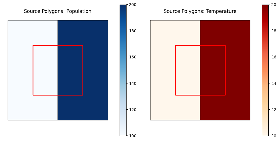
2. Visualize the Source and Target Polygons#
# Create side-by-side plots to visualize both the population and temperature distribution
fig, axes = plt.subplots(1, 2, figsize=(10, 5))

# Plot population on the left panel
source_polys.plot(column='population', ax=axes[0],
                  legend=True, cmap='Blues', edgecolor='black')
target_polys.boundary.plot(ax=axes[0], color='red', linewidth=2)
axes[0].set_title('Source Polygons: Population')
axes[0].set_axis_off()

# Plot temperature on the right panel
source_polys.plot(column='temp', ax=axes[1],
                  legend=True, cmap='OrRd', edgecolor='black')
target_polys.boundary.plot(ax=axes[1], color='red', linewidth=2)
axes[1].set_title('Source Polygons: Temperature')
axes[1].set_axis_off()

plt.tight_layout()
plt.show()
3. Compute Intersections Weights with WeightGenP2P#
# Initialize WeightGenP2P to calculate the area-intersection weights between target and source polygons.
weight_gen = WeightGenP2P(
    target_poly=target_polys,
    target_poly_idx="target_id",
    source_poly=source_polys,
    source_poly_idx="source_id",
    method="serial",              # Use serial processing for this demo
    weight_gen_crs=5070,           # Equal-area crs value
    output_file='int_ext_weights.csv',  # Save output if desired, or set to None
    jobs=4
)
weights = weight_gen.calculate_weights()
print("Calculated weights:")
weights
Calculated weights:
| source_id | target_id | source_id_area | target_id_area | area_weight | normalized_area_weight | |
|---|---|---|---|---|---|---|
| 0 | 1 | 100 | 1.986611 | 0.993306 | 0.496653 | 0.5 |
| 1 | 2 | 100 | 1.986611 | 0.993306 | 0.496653 | 0.5 |
4. Merge Source Attributes with Weights#
# To complete merge we need to cast `source_id` as str in both datasets
weights['source_id'] = weights['source_id'].astype(str)
source_polys['source_id'] = source_polys['source_id'].astype(str)

# Merge the calculated weights with the corresponding source attributes
w = weights.merge(
    source_polys[['source_id', 'temp', 'population']],
    on='source_id'
)
print("Weights merged with source attributes:")
w
Weights merged with source attributes:
| source_id | target_id | source_id_area | target_id_area | area_weight | normalized_area_weight | temp | population | |
|---|---|---|---|---|---|---|---|---|
| 0 | 1 | 100 | 1.986611 | 0.993306 | 0.496653 | 0.5 | 10.0 | 100 |
| 1 | 2 | 100 | 1.986611 | 0.993306 | 0.496653 | 0.5 | 20.0 | 200 |
5. Perform Aggregation for Intensive and Extensive Variables#
Separately compute the intensive (weighted mean) and extensive (weighted sum) aggregations.
Detailed Separation of Intensive vs. Extensive Aggregation#
# Intensive Variable Aggregation (Area-Weighted Mean)
# Multiply each temperature value by the intersection area for weighting.
w["temp_area_product"] = w["temp"] * w["area_weight"]

# For each target polygon, sum up the weighted temperatures and the total intersection area.
intensive_agg = (
    w.groupby("target_id")
    .agg(
        total_temp_area = ("temp_area_product", "sum"),
        total_area = ("area_weight", "sum")
    )
    .reset_index()
)

# Compute the area-weighted mean temperature.
intensive_agg["temp_weighted_mean"] = intensive_agg["total_temp_area"] / intensive_agg["total_area"]

# Extensive Variable Aggregation (Prorated Sum)
# For population, prorate the source's population by the fraction of its area in the target.
# The column "source_id_area" should represent the total area of the source polygon.
w["population_prorated"] = w["population"] * (w["area_weight"] / w["source_id_area"])

# Sum the prorated population for each target polygon.
extensive_agg = (
    w.groupby("target_id")
    .agg(total_population = ("population_prorated", "sum"))
    .reset_index()
)

# --- Combine Aggregation Results ---
# Merge the intensive and extensive aggregation results by target_id.
agg_detailed = intensive_agg.merge(extensive_agg, on="target_id")

# Display the detailed aggregation results.
print("Detailed Aggregation Result:")
print(agg_detailed[["target_id", "temp_weighted_mean", "total_population"]])
Detailed Aggregation Result:
  target_id  temp_weighted_mean  total_population
0       100                15.0              75.0
View intensive and extensive aggretation results separately#
intensive_agg
| target_id | total_temp_area | total_area | temp_weighted_mean | |
|---|---|---|---|---|
| 0 | 100 | 14.899584 | 0.993306 | 15.0 |
extensive_agg
| target_id | total_population | |
|---|---|---|
| 0 | 100 | 75.0 |
Summary of Results#
Given the context of intensive and extensive variables, the results of the aggregation we can understand the results as follows:
Intensive Variables: The resulting value of 15 can be understood as the average temperature across the source polygons, weighted by their area of overlap with the target polygon. Since the target polygon has equal area contributions from the source polygons, this value reflects the average temperature per unit area, which is consistent with the definition of an intensive variable.
Extensive Variables: The resulting value of 75 represents the total population across the source polygons, weighted by their area of overlap with the target polygon. Since each source polygon has an intersection area of 1/4 of the target polygon, the total population is effectively summed across the source polygons, (0.25 * 100) + (0.25 * 200) = 75hich aligns with the definition of an extensive variable. This value indicates the total number of individuals represented in the target polygon based on the contributions from each source polygon.